Examples
Geostrophic Adjustment: One-Dimension
In the directory examples you will find an example entitled
example_1D_geoadjust.py
First, libraries are imported. Two standard ones are numpy, for calculations, and matplotlib.pyplot for plotting. Those are standard to numpy. Then, there are four other things that are imported:
- Steppers This contains different time-stepping functions. At the moment we have Euler, Adams-Bashforth 2 (AB2), Adams-Bashforth 3 (AB3) and Runge-Kutta 4 (RK4). PyRsw uses adaptive time stepping to try and be more efficient in how the solution is marched forward.
- Fluxes This contains the fluxes for the RSW model. At the moment there is only the option for a pseudo-spectral model but this will be generalized to include a Finite Volume method as well.
- PyRsw This is the main library and importing Simulation imports the core of the library.
- constants This has some useful constants, more can be added if desired.
After the libraries are imported then a simulation object is created.
sim = Simulation()
Below specifies the geometry in \(x\) and \(y\): [Options ’periodic’, ’walls’]
We use AB3, a spectral method: [Options: Euler, AB2, AB3, RK4]
We solve the nonlinear dynamics: [Options: Linear and Nonlinear]
Use spectral sw model (no other choices at present).
sim.geomy       = 'periodic'
sim.stepper     = Step.AB3
sim.method      = 'Spectral'
sim.dynamics    = 'Nonlinear'
sim.flux_method = Flux.spectral_sw
We specify a lot of parameters. There are some default values that are specified in PyRsw.
sim.Ly  = 4000e3            # Domain extent               (m)
sim.Nx  = 1                 # Grid points in x
sim.Ny  = 128               # Grid points in y
sim.Nz  = 1                 # Number of layers
sim.g   = 9.81              # Gravity                     (m/sec^2)
sim.f0  = 1.e-4             # Coriolis                    (1/sec)
sim.beta = 0e-10            # Coriolis beta parameter     (1/m/sec)
sim.cfl = 0.05              # CFL coefficient             (m)
sim.Hs  = [100.]            # Vector of mean layer depths (m)
sim.rho = [1025.]           # Vector of layer densities   (kg/m^3)
sim.end_time = 2*24.*hour   # End Time                    (sec)
There is an option to thread the FFTW’s if using pyfftw.
sim.num_threads = 4
Below we specify the plotting interval, what kind of plotting to do, and the limits on the three figures.
sim.plott   = 20.*minute  # Period of plots
sim.animate = 'Anim'      # 'Save' to create video frames,
                          # 'Anim' to animate,
                          # 'None' otherwise
sim.ylims=[[-0.18,0.18],[-0.18,0.18],[-0.5,1.0]]
We can specify the periodicity of plotting and whether we want a life animation or make a video. More on this this later.
sim.output = False        # True or False
sim.savet  = 1.*hour      # Time between saves
Specify periodicity of diagnostics and whether to compute them. This is not tested.
sim.diagt    = 2.*minute  # Time for output
sim.diagnose = False      # True or False
Initialize the simulation.
sim.initialize()
Specify the initial conditions. There is an option whether we want the domain in \(x\) or \(y\). At the moment there is no difference because there is no \(\beta\)-plane but this will be added.
for ii in range(sim.Nz):  # Set mean depths
    sim.soln.h[:,:,ii] = sim.Hs[ii]

# Gaussian initial conditions
x0 = 1.*sim.Lx/2.         # Centre
W  = 200.e3               # Width
amp = 1.                  # Amplitude
sim.soln.h[:,:,0] += amp*np.exp(-(sim.Y)**2/(W**2))
Solve the problem.
sim.run()
Plot the Hovmöller diagram in time versus space.
# Hovmuller plot
plt.figure()
t = np.arange(0,sim.end_time+sim.plott,sim.plott)/86400.

if sim.Ny==1:
    x = sim.x/1e3
elif sim.Nx == 1:
    x = sim.y/1e3

for L in range(sim.Nz):
    field = sim.hov_h[:,0,:].T - np.sum(sim.Hs[L:])
    cv = np.max(np.abs(field.ravel()))
    plt.subplot(sim.Nz,1,L+1)
    plt.pcolormesh(x,t, field,
        cmap=sim.cmap, vmin = -cv, vmax = cv)
    plt.axis('tight')
    plt.title(r"$\mathrm{Hovm{\"o}ller} \; \mathrm{Plot} \; \mathrm{of} \; \eta$", fontsize = 16)
    if sim.Nx > 1:
        plt.xlabel(r"$\mathrm{x} \; \mathrm{(km)}$", fontsize=14)
    else:
        plt.xlabel(r"$\mathrm{y} \; \mathrm{(km)}$", fontsize=14)
    plt.ylabel(r"$\mathrm{Time} \; \mathrm{(days)}$", fontsize=14)
    plt.colorbar()

plt.show()
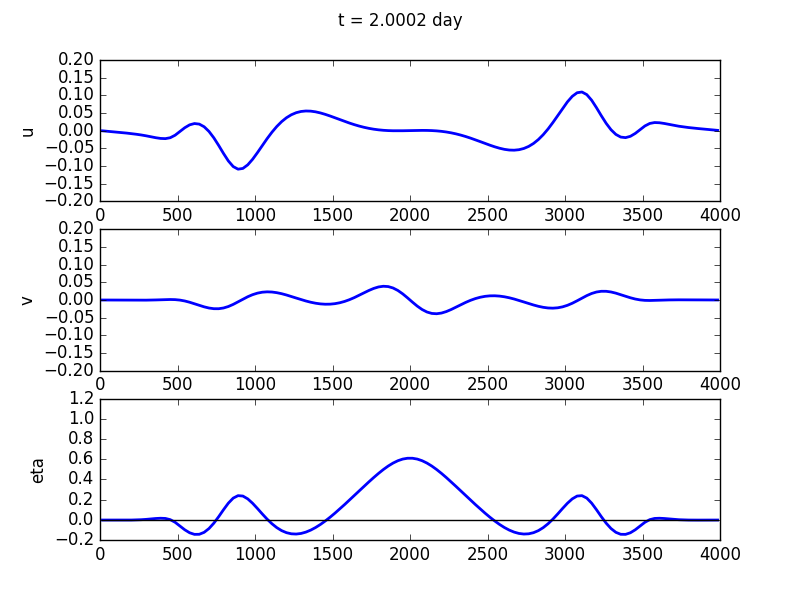
Final solution for the test case.
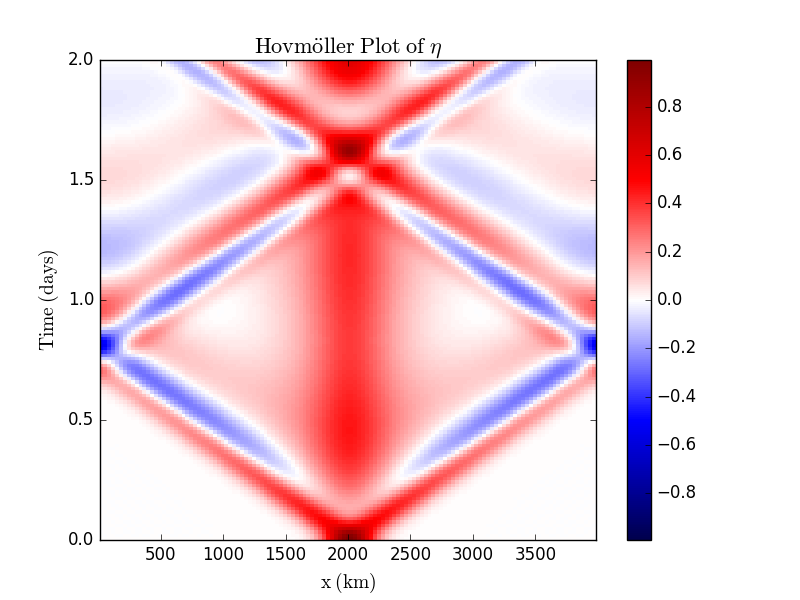
Hovmöller plot for the test case.
<<<<<<< HEAD There is a second example called example_1D_geoadjust2.py that begins with a hyperbolic tangent profile instead if a Gaussian initial condition. ======= Note that to compute the derivatives in the case of a non-periodic domain we impose either Dirichlet or Neumann boundary conditions. This is done by doing odd and even extensions respectively. That is why in 1D, the simulation with walls does twice as much work as in the periodic case. Similarly, if we have walls in 2D, that is doing four times as much work.
At some point we should change walls to ’slip’ and allow for ’noslip’ boundary conditions as well.
Geostrophic Adjustment: Two-Dimensions
The basic script is almost identical to the 1D case and can be found in the examples folder with the title example_2D_geoadjust.py. The changes are as follows:
- Set \(Nx\) and \(Ny\) both equal to \(128\), and from this we build a 2D grid.
- Specify the length of the domain in the zonal direction.
- Define the initial conditions on a 2D grid.
- The plotting is different. We plot a 2D field using pcolormesh and we don’t do a Hovmöller plot.
Bickley Jet: Two-Dimensions
Following Poulin and Flierl (2003) and Irwin and Poulin (2014), we look at the instability of a Bickley jet. The script is called example_2D_BickleyJet.py.
In this case we change the code to include the following lines.
# Define geometry
sim.geomx       = 'periodic'
sim.geomy       = 'walls'

# Define grid and domain size
sim.Lx  = 200e3          # Domain extent               (m)
sim.Ly  = 200e3          # Domain extent               (m)
sim.Nx  = 128            # Grid points in x
sim.Ny  = 128            # Grid points in y

# Bickley Jet initial conditions
# First we define the jet
Ljet = 20e3            # Jet width
amp  = 0.1             # Elevation of free-surface in basic state
sim.soln.h[:,:,0] += -amp*np.tanh(sim.Y/Ljet)
sim.soln.u[:,:,0]  =  sim.g*amp/(sim.f0*Ljet)/(np.cosh(sim.Y/Ljet)**2)
# Then we add on a random perturbation
sim.soln.u[:,:,0] +=  2e-3*np.exp(-(sim.Y/Ljet)**2)*np.random.randn(sim.Nx,sim.Ny)
>>>>>>> master
Geostrophic Adjustment: 2D and 1L
The basic script is almost identical to the 1D case. The changes are as follows:
- Set \(Nx\) and \(Ny\) both equal to \(128\), and from this we build a 2D grid.
- Define the initial conditions on a 2D grid.
- The plotting is different. We plot a 2D field using and we don’t do a Hovmöller plot.
Bickley Jet: 2D and 1L
Following Poulin and Flierl (2003) and Irwin and Poulin (2014), we look at the instability of a jet.