Examples
Geostrophic Adjustment: 1D and 1L
In the directory src you will find an example entitled
example_1D_1L_spectral.py
First, libraries are imported. Two standard ones are numpy, for calculations, and matplotlib.pyplot for plotting. Those are standard to numpy. Then, there are four other things that are imported:
- Steppers This contains different time-stepping functions. At the moment we have Euler, Adams-Bashforth 2 (AB2) and Runge-Kutta 4 (RK4). PyRsw uses adaptive time stepping to try and be more efficient in how the solution is marched forward.
- Fluxes This contains the fluxes for the RSW model. At the moment there is only the option for a pseudo-spectral model but this will be generalized to include a Finite Volume method as well.
- PyRsw This is the main library and importing Simulation imports the core of the library.
- constants This has some useful constants, more can be added if desired.
After the libraries are imported then a simulation object is created.
sim = Simulation()
Below specifies the geometry in \(x\) and \(y\): [Options ’periodic’, ’walls’]
We use AB2, a spectral method: [Options: Euler, AB2, RK4]
We solve the nonlinear dynamics (can be Linear)
Use spectral sw model (no other choices). Maybe hide this.
sim.geomx       = 'walls'
sim.geomy       = 'periodic'
sim.stepper     = Step.AB2
sim.method      = 'Spectral'
sim.dynamics    = 'Nonlinear'
sim.flux_method = Flux.spectral_sw
We specify a lot of parameters. There are some default values that are specified in .
sim.Lx  = 4000e3          # Domain extent               (m)
sim.Ly  = 4000e3          # Domain extent               (m)
sim.geomx = 'periodic'    # Boundary Conditions
sim.geomy = 'periodic'    # Boundary Conditions
sim.Nx  = 128             # Grid points in x
sim.Ny  = 1               # Grid points in y
sim.Nz  = 1               # Number of layers
sim.g   = 9.81            # Gravity                     (m/sec^2)
sim.f0  = 1.e-4           # Coriolis                    (1/sec)
sim.cfl = 0.05            # CFL coefficient             (m)
sim.Hs  = [100.]          # Vector of mean layer depths (m)
sim.rho = [1025.]         # Vector of layer densities   (kg/m^3)
sim.end_time = 36.*hour   # End Time                    (sec)
We can specify the periodicity of plotting and whether we want a life animation or make a video. More on this this later.
sim.output = False        # True or False
sim.savet  = 1.*hour      # Time between saves
Specify periodicity of diagnostics and whether to compute them. This is not tested.
sim.diagt    = 2.*minute  # Time for output
sim.diagnose = False      # True or False
Initialize the simulation.
sim.initialize()
Specify the initial conditions. There is an option whether we want the domain in \(x\) or \(y\). At the moment there is no difference because there is no \(\beta\)-plane but this will be added.
for ii in range(sim.Nz):  # Set mean depths
    sim.soln.h[:,:,ii] = sim.Hs[ii]

# Gaussian initial conditions
x0 = 1.*sim.Lx/2.      # Centre
W  = 200.e3                # Width
amp = 1.                  # Amplitude
if sim.Ny==1:
    sim.soln.h[:,:,0] += amp*np.exp(-(sim.x-x0)**2/(W**2)).reshape((sim.Nx,1))
elif sim.Nx==1:
    sim.soln.h[:,:,0] += amp*np.exp(-(sim.y-x0)**2/(W**2)).reshape((1,sim.Ny))
Solve the problem.
sim.run()
Plot the Hovmöller diagram in time versus space.
if sim.Ny==1:
    plt.figure
    t = np.arange(0,sim.end_time+sim.plott,sim.plott)/86400.

    for L in range(sim.Nz):
        field = sim.hov_h[:,0,:].T - np.sum(sim.Hs[L:])
        plt.subplot(sim.Nz,1,L+1)
        plt.pcolormesh(sim.x/1e3,t, field,
            cmap=sim.cmap, vmin = 0, vmax = amp)
        plt.xlim([sim.x[0]/1e3, sim.x[-1]/1e3])
        plt.ylim([t[0], t[-1]])
        plt.title(r"$Hovm{\"o}ller Plot\, {of} \,\, \eta$")
        plt.xlabel(r"$distance \, \, (km)$")
        plt.ylabel(r"$Time \, \, (days)$")
        plt.colorbar()
    plt.show()
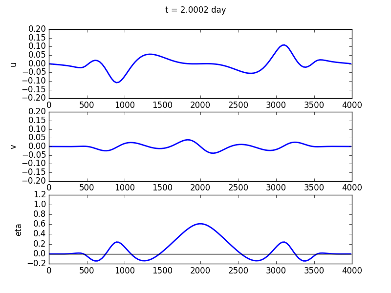
Final solution for the test case.
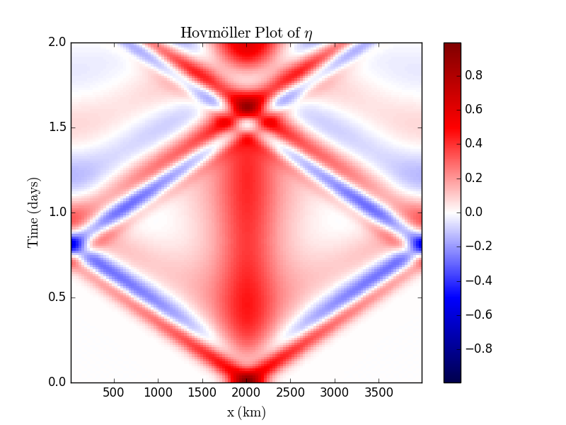
Hovmöller plot for the test case.